Segmentation Models Compared: What’s best suited to your needs?
Author: Yifei Zheng
Customer segmentation is a means of organizing and managing a company’s relationship with its customers and can improve things like personalized marketing communications, customer service and support efforts, customer loyalty, identifying the most valuable customers, and identifying new product or upsell opportunities. This can be an extremely valuable asset to any company, but building an effective segmentation model can be challenging.
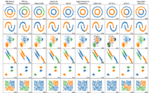
A generalized framework for building a customer segmentation model, like the one in our previous blog post, can be beneficial when beginning this process, but what about the technical considerations? Approaching such a task from a business standpoint with a generalized framework to follow is a great start, but it’s only half of the puzzle. The second half involves determining what kind of model you will use to segment your customers. For this, we’ll need to look at each type of common segmentation model individually and weigh the pros and cons of each. Some of the most common models, and the ones we’ll be covering here, are:
- K-Means Clustering
- DBSCAN
- Affinity Propagation
- Gaussian Mixture Model (GMM)
- Agglomerative Hierarchical Clustering
Below, we’ll examine each one individually to help you identify which is best suited for your needs.
K-Means Clustering
K-Means Clustering is a type of centroid-based clustering method and is the most well-known and widely-used segmentation method. The term centroid is another name for the mean of data points in a given cluster. K-Means Clustering aims to separate your data into K disjoint clusters by choosing centroids that minimize the inertia criterion, which in essence, tries to make each obtained cluster as internally coherent as possible. K-Means Clustering is a reasonable starting point for most forms of customer segmentation projects. It is easy to implement, can scale to large datasets, and can be applied directly to new data points to assign them to their most suitable cluster. The algorithm is also guaranteed to converge, so you’ll always end up with a set of clusters for your data.
In addition to all these characteristics that make the K-Means method attractive, there are several drawbacks to consider as well. Firstly, K-Means requires you to specify the exact number of clusters to look for in their data (i.e. the value for K), and you could end up with non-sensible results if the value for K you chose is too far from the actual number of clusters in the data. Additional analysis around how within cluster losses vary with the number of clusters is recommended to select the optimal value for K.
Another thing to keep in mind is the potential instability of clusters obtained by running K-Means. Because the algorithm initializes the centroids randomly, it’s possible that a particular run will get stuck in a sub-optimal local minimum, so it’s usually a good idea to run the algorithm multiple times with different initial values for the centroids and pick the one that gives the best clustering fit. Finally, when the dataset you have contains a large number of dimensions, it’s preferable to first run a dimension-reduction algorithm such as Principal Component Analysis (PCA) before applying K-Means, since it becomes increasingly difficult for K-Means to correctly measure the similarity between two data points as the data dimensionality increases.
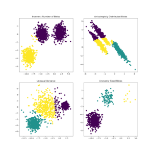
K-Means Clustering is usually the first segmentation algorithm to explore, and it can often produce very good results. However, the way this algorithm was designed implies that it will not perform perfectly for every type of dataset. Specifically, when the true clusters in your dataset have varying shapes, sizes, and densities, or when there is a significant number of outlier data points that don’t form nicely into clusters, it’s a good idea to turn to a density-based clustering algorithm.
DBSCAN
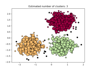
Density-based spatial clustering of applications with noise, or DBSCAN, is a density-based clustering algorithm that takes the general approach of viewing clusters as areas of high densities surrounded by areas of low densities. This general view allows DBSCAN to identify clusters of any shape, marking an improvement over K-Means in this aspect. Aside from the actual clusters, DBSCAN also classifies each data point into three types:
- Core points, which are near the center of their respective clusters and are the most typical representations of a cluster
- Non-core points, which are near the periphery of a cluster but still part of the cluster
- Outliers, which are points in the low-density regions separating the clusters.
This more detailed separation of individual data points is helpful for creating finer-grained marketing and ad campaigns to target customers closest to a specific profile.
The added flexibility of the DBSCAN algorithm comes at a cost. Implementation of DBSCAN is memory-intensive and requires a large amount of resources to run on large datasets. The hyperparameters that define the high/low-density regions require tuning as well. Finally, DBSCAN is not designed to apply directly to new data points, so a separate classifier is usually needed to make predictions.
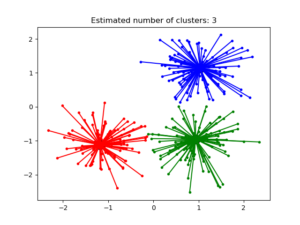
Affinity Propagation
Affinity Propagation is a clustering model based on the concept of “message passing” between data points. It creates clusters through voting where data points vote for similar instances to be their representatives until convergence. Affinity Propagation is similar to DBSCAN in that it also handles clusters of varying sizes and shapes and requires tuning of certain hyperparameters to achieve the best results. The main drawback of Affinity Propagation is its time complexity, which is on the order of N^2, with N being the number of data points in your data, making it only suitable for small to medium-sized datasets. Affinity Propagation can scale up to a large number of clusters in the data and can be directly applied to new data coming in.
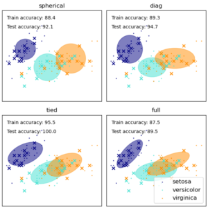
Gaussian Mixture Model
Gaussian Mixture Model, or GMM, is a probabilistic model that assumes all the points in your data are generated from a mixture of several Gaussian (i.e. Normal) distributions with unknown parameters that can be estimated from the data. This algorithm can be viewed as an extension of the K-Means Method because it treats each cluster as a Gaussian distribution component while further incorporating information about the centers of these distributions and the covariance structure of the data when determining the optimal cluster separations. Being a probabilistic model, GMM produces ‘soft assignment’ by giving each data point probabilities for belonging to the different clusters. It can also be applied directly to new data observations. The downsides of this approach include the following:
- A greater need for data to accurately estimate the parameters of the underlying Gaussian distributions (preferably many data points with low dimensions)
- The need to specify the number of Gaussian distribution components (akin to K-Means)
- Reduced effectiveness in modeling non-ellipsoidal clusters in the data since they don’t follow model assumptions.
Agglomerative Hierarchical Clustering
Agglomerative Hierarchical Clustering is the most common type of hierarchical clustering used to group objects in clusters based on their similarity. It’s also known as Agglomerative Nesting or AGNES. As the name suggests, Agglomerative Hierarchical Clustering works by starting from each data point as its own cluster and successively merging the clusters in a bottom-up fashion. There are a number of criteria (linkage) to determine the merging of the clusters, and the choice of the linkage will impact the final clustering results, so it is recommended to investigate and compare the results obtained with different linkages. As a rule of thumb, single linkage clustering, which merges clusters by minimizing the distance between the closest points in a pair of clusters, can be computed very efficiently and so is scalable to very large datasets, but at the same time, is also more vulnerable to noisy outliers in the data.
One added benefit of the Hierarchical Clustering approach, especially for smaller datasets, is the ability to visualize the entire cluster hierarchy, showing how the individual clusters successively merged to become a single, all-encompassing cluster. This hierarchical view can help provide a more holistic understanding of the structure inherent in the data and, in turn, aid the decision of the optimal number of clusters to use from a business perspective.
There are many different segmentation models, each with unique attributes that make them ideal for different kinds of data and business initiatives. Equipped with the knowledge included above, you can find the one that’s best suited for your needs by performing an EDA, selecting several clustering algorithms based on what the data looks like, running them, comparing the results and then combining these results with business considerations before iterating on the process. For more information about customer segmentation models and other data science related topics, follow our blog or contact us directly to discuss your unique needs.