An Examination of Distribution Prediction Methods

Author: Konstantin Galperin

The current supervised machine learning toolkit is vast, and such methods are applied with a single goal in mind – making a point prediction. However, in some cases, it might be beneficial to predict a range of outcomes. For example, an insurance company might find it beneficial to forecast not only an average claim amount but also the occurrence and magnitude of large claims, since they can be rather influential on the business. In mechanical systems, a process that utilizes a normal load should be sustained by the system indefinitely, while an outlier may cause the system to fail. An irregular load might not cause a system failure, but it could impose stress on the system, thus reducing its lifespan.

For such cases, it might be beneficial to make a distribution prediction. Some of the standard methods might have a distribution prediction built in, such as confidence intervals in a regression. Here, however, we try several methods that are more generic and can be used across various estimation methods which produce a continuous point prediction.

Methods

We used 3 methods: non-parametric bootstrap, parametric bootstrap, and histogram prediction. We applied these to several datasets, both real-world and simulated, to test their effectiveness and foresee shortcomings of typical modeling processes.

Non-parametric bootstrap steps:

Split data into train and test sets
Resample. Create B bootstrap samples by sampling with replacement from the train data. Each sample of the same size as training data
Fit a separate model to each sample
Project. Create B projections from test data
Evaluate predictions. For each input point in the test data we now have B outputs. One can compare how many dependent actuals fall within a certain percentage of this projected distribution. I.e. are 95% of actual dependent values within 95% of projected distribution etc.

Parametric bootstrap steps:

Split data into train and test sets
Fit single model on whole train data
Produce B projections on test data by either a) assuming an error structure. In the models discussed here, we assume the error is additive and normal with 0 mean and standard deviation derived from the fitted model. Then simulate outcomes by getting fixed projection from the model and adding values drawn from the error distribution. Or b) if the fitted model projection by design draws from random variables, then simply run B projections
Evaluate predictions the same way as in non-parametric bootstrap

Histogram prediction steps:

Split data into train and test sets
Create a histogram from train dependent – i.e. assign train data into M bins. Note that bin selection is extremely important and domain-specific.
Create M dummy variables taking a value of 1 if a dependent in a particular bin and 0 otherwise
Train a neural net with softmax output (or other model).
Evaluate predictions

Examples

Real-world datasets were obtained from UCI machine learning repository. We used 3 different datasets, with the idea of producing a good-fitting model, a mediocre-fitting model, and a poorly fitting model. By applying the non-parametric bootstrap, parametric bootstrap, and histogram predictions, we can observe how the methods behave in each case.

The datasets are:

Plant energy output. Features consist of hourly average ambient variables Temperature (T), Ambient Pressure (AP), Relative Humidity (RH), and Exhaust Vacuum (V), and the goal is to predict the net hourly electrical energy output (EP) of the plant.
Hourly Minneapolis-St Paul, MN traffic volume for westbound I-94. Features are transformed using standard techniques and include holidays, weather, weekday, and hour. The goal is to predict traffic volume
Protein structure data. Features consist of 9 measures of protein structures. And the goal is to predict RSMD – root-mean-square deviation of atomic positions

Standard preprocessing was used such as coding categorical variables as dummies and dropping observations with missing values. For histogram prediction, bins were mostly equally spaced across dependent ranges. OLS was used in both bootstrap methods. Since parametric bootstrap requires a distribution assumption for errors, normal distribution was assumed with 0 mean and variance equal to MSE from the fitted model. We can obtain point predictions from them by taking the average of the outcomes. And so computing MAPE then produces the following:

	Energy Output	Traffic Volume	RSMD
Non-Parametric Bootstrap MAPE	0.8%	27.03%	88.69%
Parametric Bootstrap MAPE	0.802%	29.37%	115.19%

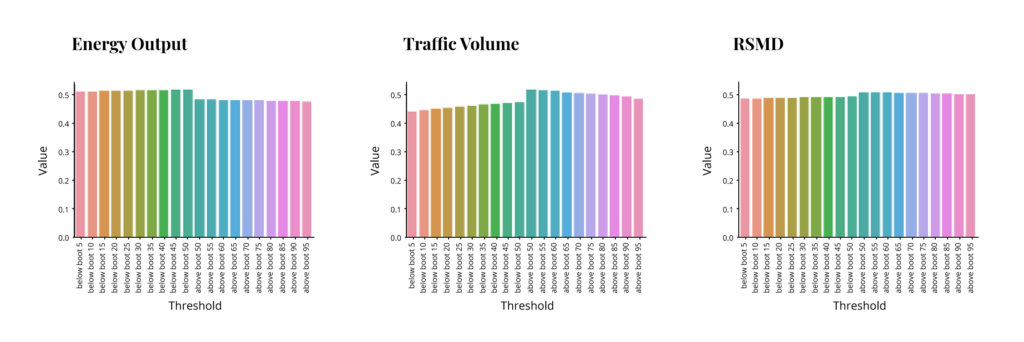
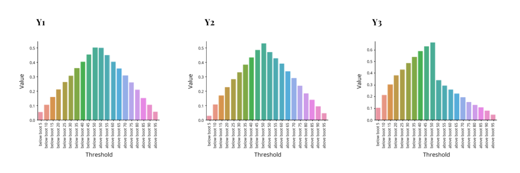
So we have 3 different models with substantial differences in quality of fit. Now the question is how distribution predictions behave in each of these. We evaluate the performance by comparing how many of the dependent values actually fall within a certain percentage of the projected distribution. I.e. are 95% of actual dependent values within 95% of projected distribution etc. Each of the following graphs shows the percent of dependent distribution on the y-axis corresponding to the percent of projected distribution on the x-axis. The left half of the x-axis for each graph has percents below some threshold (5,10,15 etc. through 50), while the right half has percents above a threshold (50 through 95). The ideal outcome would be that the y values match the threshold on the left side and match “1 – the threshold” on the right side, resulting in a symmetrical pyramid with two middle points at .5 and the rest decreasing at a 45-degree angle. These are the results for each method.

Non-Parametric Bootstrap:

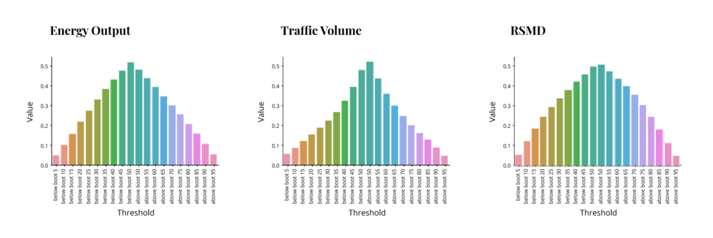
Parametric Bootstrap:

Histogram Prediction:

As we can see, non-parametric bootstrap fails completely to capture distribution, while histogram prediction is perhaps acceptable for the energy output model but struggles in the other two. The first is actually expected, and the second depends on bin selection, which was rather simplistic in this case. Interestingly the parametric bootstrap performed rather well in all 3 models. This was expected for the good fit model, but the poor fit model outcome is not guaranteed, as we shall see later. And so, this speaks to the robustness of the method.

Simulated Data

In addition to the real-world data, we tried models on simulated data. Here we can test distribution around independent points. I.e. in real-life data, there are usually little to no duplicates in a set of independent variables, so we cannot observe how the dependent varies around fixed independents. But we can with simulated data

The simulation process was done in 3 steps:

Simulate several random variables with fixed size (10000 rows). Going forward assume all but one of these is fixed, and the other one is random. The fixed portion is now X, and the random variable is error.
Produce Y according to some equation. The set of Y and X is now a simulated version of what is typically available in real-life applications.
Using the same fixed X, redraw a random variable corresponding to error and recompute Y. Repeat multiple times (1000). The collection of new Ys (10000 x 1000 matrix) is now a distribution of the dependent given fixed X.

Here we will go over 3 examples. Last term in each is error:

Y1 = 5 + 300*uniform(0,1) + normal(0, 1).
Y2 = 5 + 100*uniform(0,1) + 5*correlated_gamma(1,2) + 3*correlated_gamma(1,1) + burr(7,0.2).
Y3 = 5 + normal_mixture_beta * (correlated_invweibull_1(200) + correlated_invweibull_2(200) + joint_normal(-5,.2,-.2) + joint_normal(4,.25,-.2) + chi_square(15))

The approach is similar to the one taken before. We have models, the first is expected to fit really well (here it is guaranteed by the setup), the second might fit well, the last one will not. The issue is, of course, that the correct distribution is known in advance, so we only tried standard methods that an analyst might try by simply looking at the dependent distributions while not knowing what the error terms are or how they are related to the dependents. Note that in the last model, error is neither typically additive nor can it be easily made into such via log transform.

The first two models were fitted using OLS. For the last model, regression fits were poor, although ridge regression performed better than OLS, and log transformation performed better than the original dependent. So, Mixture Density Network was used.

Similar to the first set of models, here is MAPE summary:

	Y1	Y2	Y3
Non-Parametric Bootstrap MAPE	3.117%	2.17%	34.2%
Parametric Bootstrap MAPE	3.123%	2.19%	35.4%

Evaluating the outcomes same as earlier:

Non-Parametric Bootstrap:

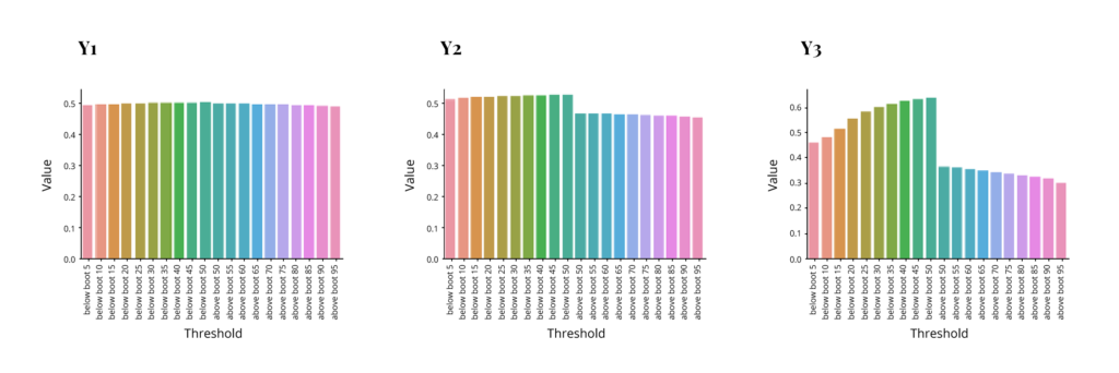
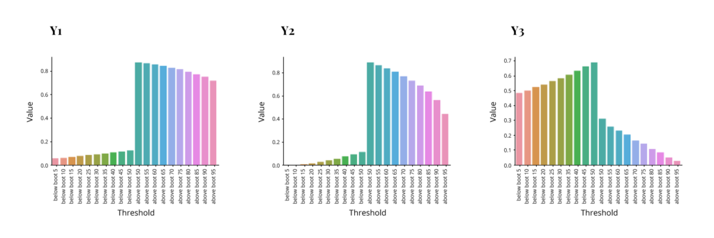
Parametric Bootstrap:

Histogram Prediction:

Conclusions

Some key takeaways from the above exercise are as follows:

Parametric bootstrap worked best in the attempted models. Normal errors were assumed in all cases, and it appears to produce adequate results if errors are additive, even if they are not particularly normal. If, however, the errors structure is too complex, none of the methods works well
Histogram didn’t work as well, but often performed better than non-parametric bootstrap. Bin selection appears to influence results a lot – for example, going from bins with the same number of observations to bins with more or less equal support range produced big changes in one of the simulated models.
Non-parametric bootstrap often produced best point predictions

Overall parametric bootstrap appears to perform well. The method is easy to implement and can be combined with a variety of machine learning methods. It should probably serve as a first choice for distribution predictions. While histogram prediction didn’t work as well, there is certainly a possibility that it would outperform parametric bootstrap in some tasks where the bootstrap modeling is challenging and there is substantial domain knowledge. Follow our blog for more information on distribution predictions and other data science-related topics or contact us directly to discuss your unique needs.