An Introduction to Network Analysis

Author: Igor Pshenychny

A network analysis is a means of understanding the various entities of a given dataset as well as the relationships between them. It is a useful tool that can generate unexpected insights even when the dataset doesn’t seem conducive to a network analysis. This is because every dataset is composed of entities that are related to one another in various ways.

Customer data sets can show geographic relationships between products or identify trends in shopping behavior
Within the context of website traffic, a network analysis can show influential links that connect various communities to a specific brand/product
Within an email network you can measure influential individuals that are critical in maintaining the flow of information, or popular individuals who hold the most information
Within the context of protein interactions one can map the physical interactions between specific proteins to deepen our understanding of human disease

Below we’ll show some examples of how to perform a network analysis, explain some important metrics that could lead to interesting insights, and discuss the pros and cons of popular visualization techniques found in the Python package NetworkX.

How would one begin an analysis?

The first step when performing a network analysis is to ask yourself two questions:

What are the entities you want to examine?
What lens would you like to view the relationships from?

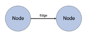
The first question highlights the basic components of a network analysis. The entities you examine will be the “nodes” or points of contact for your graph while the connection or relationship between nodes is called an “edge”. The second question is important to consider because a given dataset can be analyzed in multiple ways. For example, when analyzing the US domestic flights and airport dataset, you can look at a network through the lens of the number of planes arriving and leaving, the number of passengers traveling, the amount of cargo transported, the amount of medical equipment/supplies delivered, the various carriers traveling to that node, or the time of flight.

Based on your answers to these questions, the next step is to create a graph with your data. A common way of creating a graph using the NetworkX module is by using the .from_pandas_edgelist method, but you’ll first need to structure your dataframe to ensure the source and target are what they should be.

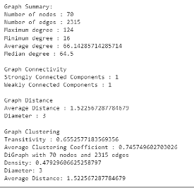
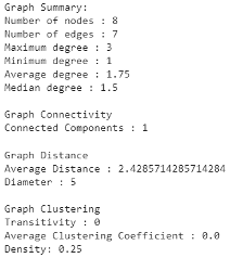
Once you have your graph, the next thing you want to do is look at the statistics of the entire graph including the number of nodes, the number of edges, and the Maximum degree (the score of a node, aka how many edges are connected to the node). NetworkX provides various functions to output these statistics and more.

Graph Statistics

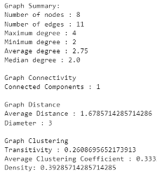
Graph statistics can paint a quick picture of the data by highlighting things such as density, connected components, and diameter.

The Density of a graph shows the ratio of edges that exist within the graph to maximum total possible edges that can exist. This metric is calculated by Gaussian Sums which tells us the total possible number of edges that can exist is V(V-1)/2, and so the density of a graph would be 2E/(V*(V-1)) where E and V represent the number of nodes and edges respectively. For a directed graph, where a connection between node1 to node2 isn’t the same as a connection between node2 to node1, then the formula is adjusted to become E/(V*(V-1))

Average Degree tells us how many connections one would expect a node to have within the graph.

Diameter tells us the distance or length of the path between the two farthest nodes. In the context of the US domestic flights and airport dataset (shown above) we can see that the diameter of the graph is 3, meaning that there exist two airports that must require 3 separate flights in order to travel from one to the other. If you were to consider taking every node in a graph and placing it on the circumference of a circle, then the nodes that are the most separated should ideally be located on antipodal points, making the distance between them the diameter.

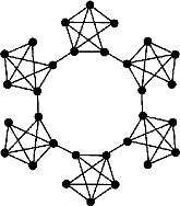
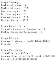
Average clustering coefficient shows the average percentage a group of neighbors is away from being a completed graph (a clique where all nodes are connected with each other). This is a measurement of how likely our friends/neighbors are also friends/neighbors with each other. In the 3 graphs shown below the average clustering coefficient increases from 0 to 0.33, then to 0.64 as we connect more edges together. Do not confuse this with the density of a graph. With each graph one can see the chances of finding a tightly knit community increases. Here is an example of a graph with a high average clustering coefficient but low density:

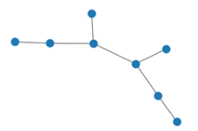
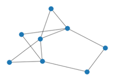
These statistics can be incredibly useful when trying to understand your data, especially when the dataset in question is much too large to view graphically. In order to get a sense of how much variation there can be between graphs and their related statistics, we’ve included a few example graphs that have a manageable size of 8 nodes.

Node Statistics/Graph Centralities

All of the previously mentioned statistics describe a network analysis graph as a whole but each of the nodes also have important and illuminating statistics. Graph centralities refer to a group of node level statistics that are important because they provide a unique perspective and are a treasure chest of insights. Below we’ll break down some of the most important graph centralities that you should include in your analysis.

Degree Centrality: A simple measure of how many neighbors a node has. It can help identify popular entities and can serve as an estimate for the center of clusters within the network.

Betweenness Centrality: Nodes with a high betweenness score are essentially bridges that connect different clusters. This can be used to measure the influence of a node. By considering all possible shortest paths that connect any two separate nodes in the graph one can ask, how many times is one particular node included within all possible paths? If the node is included in about 1% of all the paths connecting nodes together, it won’t have a high betweenness score. Conversely, if that particular node is present in 90% of all paths connecting any two nodes together, then it’s betweenness centrality will be high. The frequency with which a node appears within all shortest paths between every two nodes determines it’s betweenness score.

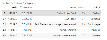
Closeness Centrality: This tells us the most influential nodes that can distribute information to the whole network with the least number of steps. This can also be useful to show the shortest path between the lowest closeness nodes. Getting an estimate of the maximum number of steps one would need to take in order to reach from one part of the network to another aka the diameter. The closeness score will represent the inverse of the distance you’ll need to travel to get from one node to another and is the average metric for how close you are to other nodes.

Eigenvector Centrality: A metric that is similar to degree centrality but it also considers the number of neighbors your neighbors have, as well as the number of neighbors those neighbors have, and the number of neighbors your neighbor’s neighbor has. After counting these values, it’s calculated again and again, constantly being normalized until the values for the centrality converges.

Pagerank Centrality: PageRank’s main difference from Eigenvector Centrality is that it accounts for link direction. Each node in a network is assigned a score based on its number of incoming links (its ‘indegree’). These links are also weighted depending on the relative score of its originating node.

The relationships/correlations between these metrics generate insights as well. If the centralities are closely related to one another then it usually describes a graph very close to being a complete graph, a graph where every node is connected with each other. A scatter plot of degree score versus betweenness score can highlight nodes with high betweenness score but low degree centrality, signifying bottlenecks within the network. For example, an airport that connects cliques or networks together, like Ted Steven’s international airport [1] connecting the clique of United States airports to Russian and Chinese airports.

Each of these metrics highlights a single perspective of the entire graph and only shows you one picture of that network. Graphs can be massive and hard to reason with. These metrics are a means of getting a different but important perspective. Adding in additional metadata and assigning weights to edges can uncover even deeper insights and running through more centrality metrics can highlight those important insights.

Popular Visualizations within NetworkX

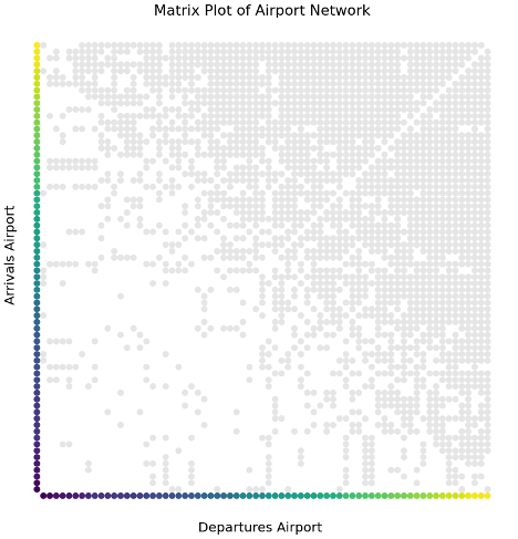
Matrix Plot:

A very popular and useful visualization in NetworkX is the Matrix plot. This is a grid that has an X and Y axis consisting of every node in the network. An edge, or connection between any two nodes, is represented by a dot at the X and Y coordinates of the connecting nodes. For example, a dot at the coordinates (A, B) would denote an edge between node A and node B. This method of visualization can be very useful, especially If you order the nodes by degree score which will allow you to visualize clusters and estimate density between collections of nodes.

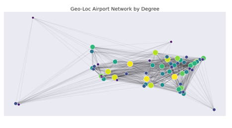
Geolocation:

Another popular option is to graph by geolocation with color representing the degree score. Using the above example of flight traffic for all US national flights, we can see that the airports in the middle of the US have higher degree scores which means they serve as transfer stops. The connectivity of these airports is higher for mid-states and the very close relationship with betweenness centrality shows that these are also networks that are centers of east and west cliques/clusters. We can also see that flights with the lowest degree centrality are geographically far away and are usually connected to high degree centrality airports.

Performing a network analysis on any given dataset will lead to insights that may not be uncovered otherwise. The statistics produced from such an analysis allow you to gain perspective about the relationships between the various components that make up a dataset, even when the given dataset is too large to graph visually. If you want to learn more about network analyses or other data science related topics, make sure to follow our blog. If you have a question about your specific needs, contact us today.